Step 5: Estimate Stressor-Response Relationships 

Simple linear regression is the recommended approach for estimating relationships between stressor and response within groups of water bodies. The straight line that relates stressor and response is easily communicated and interpreted, and is applicable to a wide variety of different variables. You can find basic assumptions underlying linear regression in NIST/SEMATECH 2013 EXIT.

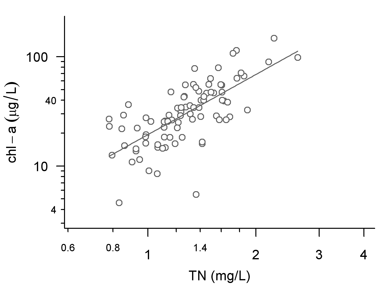
Figure 5. Example of simple linear regression used to estimate stressor-response relationship. A straight line can be described by two parameters: the slope and the y-intercept.

Regression analysis provides an estimate of mean relationship in the form of a slope and intercept of a straight line. It also provides an estimate of variability of response for the mean relationship (residual variation). In Figure 5, this variability can be visualized as the scatter of sample points around the mean line.

Analyses that begin with linear regression can be refined as needed. For example, more complex statistical analysis can estimate the magnitude of different contributions to residual variance (e.g., sampling or temporal variability). You can use that information to better understand effects of different criterion values (Yuan and Pollard 2015b). In other cases, simple linear regression can be refined to account for other types of data distributions:

• A response variable that can be expressed as a yes/no response (e.g., are algal blooms present or absent?) can be modeled as a Bernoulli distribution Exit.
• A response variable that can be expressed as a count (e.g., the number of species present) can be modeled as a Poisson distribution EXIT.

Step 6: Derive Criteria

Once you have estimated the stressor-response relationship, you can calculate the nutrient criteria. First, select the desired level of the response variable. For example, the maximum concentration of microcystin in drinking water to protect children has been established in an EPA Health Advisory as 0.3 µg/L. Another example might be the dissolved oxygen criterion for warmwater fish of 4 mg/L. After setting the desired response level, use the estimated regression relationship to estimate mean concentration of stressor necessary to achieve the desired threshold for the response variable (i.e, mean criterion value) (see Figure 6).

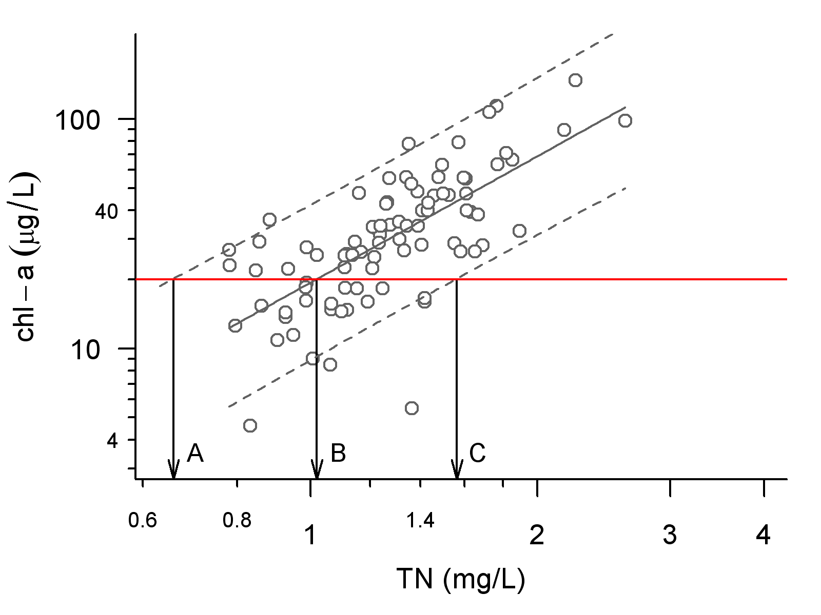
Figure 6. Prediction intervals can provide a range of different possible criterion values, each associated with a different probability of different response values. Criterion B is associated with chlorophyll a exceeding the threshold of 20 μg/L in 50% of samples. Criterion A is associated with chlorophyll a exceeding the threshold in 5% of samples. Criterion C is associated with chlorophyll a exceeding the threshold in 95% of samples.

After calculating the mean criterion value, it is often useful to quantify the uncertainty about the mean value (see Figure 6). Using linear regression, you can compute prediction intervals that define the range of possible values for a single additional sample. Criterion values associated with the intersection between the response level and different prediction intervals can then provide insights into the range of possible outcomes associated with different criterion values. For example, you would infer that, in lakes with TN concentrations at “A” in Figure 6 (based on the intersection of the upper 95th prediction interval and the response level), only a 5-percent probability exists of a future sample to exceed the response threshold.

To assess the potential effects of other unmodeled factors, reconsider the conceptual diagram. Were candidate classification variables identified in the conceptual model, but not considered in the analysis? If compelling evidence exists that a particular classification variable is important (e.g., in other studies), then gathering more data on that variable might be useful in reducing the uncertainty of the final criterion values.

Step 7: Evaluate and Document Results

Thoroughly evaluating and documenting the results of the analysis are critical for communicating the results to stakeholders. In the evaluation phase, consider whether the final criterion (and associated stressor-response relationship) is sufficiently precise to inform management decisions. One way to make this determination is to examine the range of possible outcomes associated with a particular criterion value and assess whether the different environmental outcomes are acceptable. In Figure 7, arrow B indicates the TN criterion based on the least sensitive lake. The dashed arrow indicates the prediction of the mean chlorophyll a concentration at the most sensitive lake for this criterion value. So, managing to a mean chlorophyll a concentration of 20 µg/L in the least sensitive lake could result in a mean chlorophyll a concentration of approximately 50 µg/L in the most sensitive lake. Environmental managers might or might not find that range of outcomes acceptable.

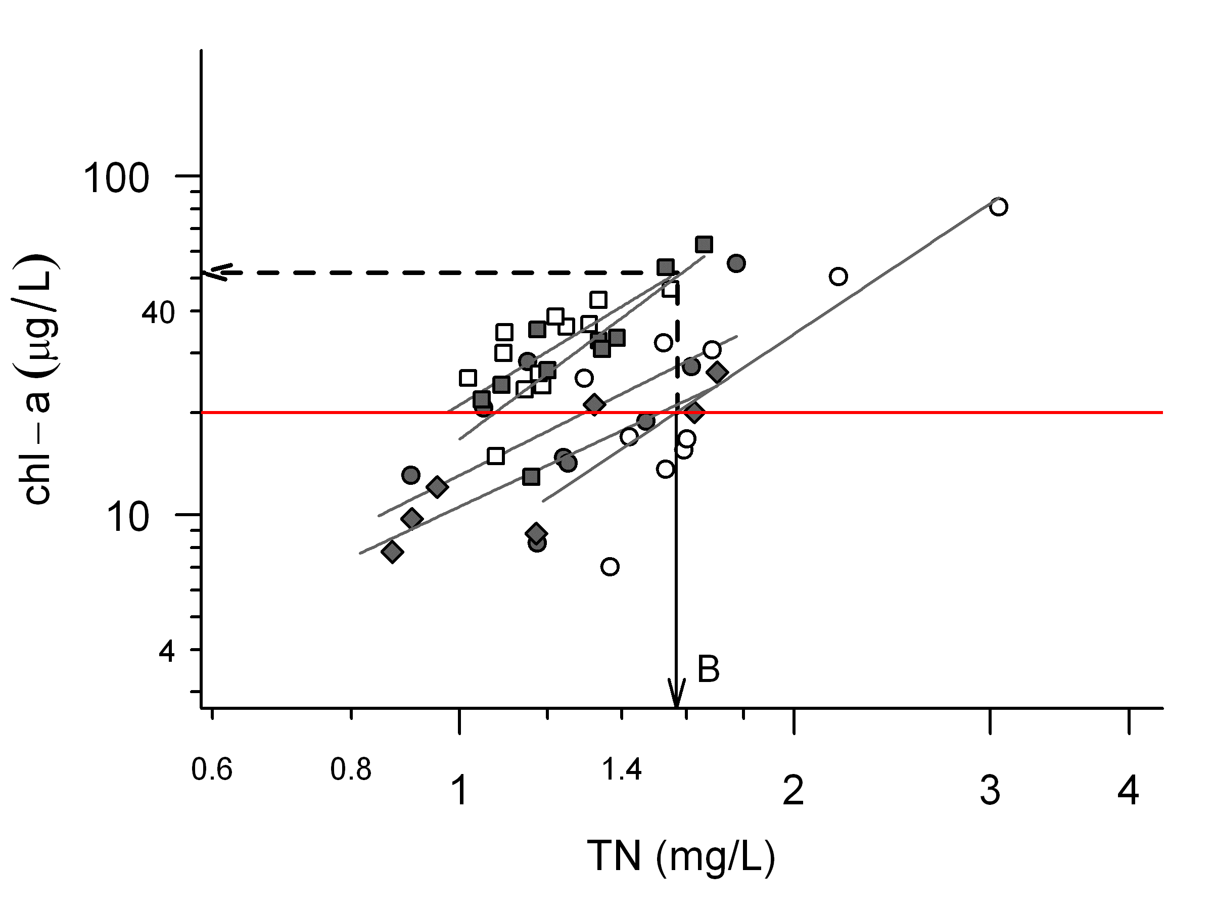
Figure 7. Illustration of range of chlorophyll a values associated with a selected criterion. Different symbols correspond to data from different lakes. Lines show relationships estimated in each lake.

Ideally, every aspect of the analysis should be documented so that independent reviewers can understand the decisions and choices made during the analysis. In particular, analysis decisions that influenced the final results should be recorded. Other items that should be documented include data sources, the process by which primary and classification variables were selected, and the rationale for the final classification approach. Statistical summaries of the stressor-response relationships also should be provided as well as the calculations used to derive final criterion recommendations.