
Data Considerations
Selecting Variables
Your focus is on two types of variables: primary and secondary. Primary variables are used to evaluate or predict the trophic status or degree of nutrient enrichment of waterbodies, especially when compared with reference conditions. They are your criteria variables. They include causal variables, typically, total phosphorus (TP) and total nitrogen (TN) and one or more response variables. We expect that the magnitude of response variables changes with changing levels of nutrients, and would provide evidence of whether the designated use of the waterbody is supported.
All other variables are secondary variables, and the nature of these variables depends on the approaches you use to develop the nutrient criteria. For example, when using the reference condition approach, you may need specific variables that help predict naturally occurring nutrient concentrations in different reference waterbodies. In contrast, when using a stressor-response approach, secondary variables will be selected based on whether they influence estimates of relationships between your causal and response variables. In this latter case, you will use the conceptual model you developed in the Problem Formulation Phase to identify secondary variables because it identifies variables that can potentially influence the stressor-response relationships of interest.
Do not confuse primary and secondary variables with primary and secondary data. Primary data are collected by your agency in the field specifically for input into your nutrient criteria development process. Secondary data, on the other hand, are existing data collected by others, for a purpose other than developing criteria. Primary data collection requires a substantial investment of time and money and, may be initiated only if critical gaps are found in secondary data sets. Since you probably will be using mostly secondary data, these data are the main focus of this section.
You should carefully examine candidate secondary data sets and evaluate if they were collected with sampling designs and methods that are compatible with your needs. Key to answering this question are metadata, which, in general, include:
- Data collection details such as location, date and time of measurements, and sample depth,
- Instrument details that include manufacturer, model, and sampling rate,
- Data sampling and processing details such as field methods and protocols and quality control (QC) procedures, and
- Analysis details such as laboratory methods and procedures and quality assurance (QA) procedures.
The availability and quantity of suitable secondary data may influence your selection of variables. If data is insufficient for a desired variable, you may have to abandon it and select an appropriate surrogate. Keep in mind that variable selection is usually an iterative process; you will likely revisit and revise your variable list as you work through the various steps of developing the criteria and collect different types of data.
Variables associated with different freshwater and marine resources are discussed.
Freshwater Resources
Classification variables
Classification is an important step in reducing variability within a distinct water body class. The ecoregion approach generally serves as a starting point for classifying freshwater resources. The geographic divisions are based on interpretations of the spatial coincidence of geographic phenomena that cause or reflect differences in ecosystem patterns (e.g., geology, physiography, soils, and hydrology). Other classification variables for lakes and reservoirs include:
- Size variables such as area of water surface or watershed. A volumetric variable such as mean or maximum depth is sometimes used for further subgroupings.
- Origin (e.g., glacier, volcanic), which affects the area, volume, and shape of natural lake basins.
- Intrinsic (or nonnutrient) water chemistry, typically dissolved organic matter (DOM), conductivity, or water color or acid-based variables (e.g., alkalinity, pH) because they are reflective of geologic conditions and inflow sources.
Reservoirs may be considered separately from natural lakes when data suggests fundamental differences between the two in your region. In general, reservoirs are most numerous in regions with few or no natural lakes, however. Reservoirs can be classified by several factors associated with hydrology or morphometry and even management objectives. Reservoir age also is a consideration due to their gradual fill of sediments.
Classification variables for rivers and streams include:
- Fluvial geomorphology (e.g., stream channel dimensions, water discharge and sediment load, and size characteristics).
- Stream order is used to classify streams within a watershed and provides a generally accepted method for distinguishing wadeable from nonwadeable streams.
- Hydrologic and channel morphological variables often are important measurements because they affect algal biomass (e.g., large stable rocks generally have higher periphyton biomass).
- Flow conditions, including low and stable flow levels and frequency and timing of floods, also affect the algal community.
Nutrient enrichment and primary productivity-related variables
The conceptual model can provide guidance on secondary variables that might be important in your analyses, especially if you are using the stressor-response approach. They include variables associated with:
- Point source compositions and emission rates (e.g., municipal wastewater, industrial wastewater, and confined animal feeding operations),
- Nonpoint source compositions and emission rates from urban, agricultural, and other land uses (e.g., fertilizers, animal feces, and nutrient-enriched sediments),
- Underlying geology (e.g., alkalinity, conductivity, and pH),
- Fractions of N and P (e.g., total inorganic N, total organic N, total Kjeldahl N, NO2/NO3, NH4, total P, PO4, and N and P loading estimates),
- Lake characteristics (e.g., retention time, lake depth, and stratification) that affect flushing rates and internal nutrient cycling,
- Light and temperature variables (notably, color and suspended sediments in a lake can change the light available for photosynthesis),
- Frequency and intensity of harmful algal blooms, and
- Indices of biological integrity.
Metadata and sampling considerations
Lake and reservoir sampling can vary from single-site sampling (often the deepest point of the lake) and multiple-site sampling to spatially composite samples from multiple locations in a lake and multiple sections of large lakes. You need to carefully review metadata to evaluate the data set compatibility. Ideally, lakes will have been sampled once during an index period that characterizes their nutrient or trophic state (e.g., during spring overturn) and with sampling methods that are assumed to characterize the lake (e.g., pumped or composite samples of the entire water column). Some data sets might support estimating annual or growing season average nutrient concentrations.
Once you have selected stream reaches for data collection, you must identify temporal periods for collection. Nutrient and algal problems frequently are seasonal in streams and rivers, so you can target sampling periods to the seasonal periods associated with nuisance problems. Nonpoint sources could cause increased nutrient concentrations and turbidity or nuisance algal blooms following periods of high runoff during spring and fall, while point sources of nutrient pollutants might cause low-flow plankton blooms and/or increased nutrient concentrations in pools of streams and in rivers during summer. Alternatively, sampling should be conducted during the growing season at the mean time after flooding for the system of interest. Algal blooms, both benthic and planktonic, can develop rapidly and then can dissipate as nutrient supplies are depleted or flow increases. Thus sampling through the season of potential blooms might be necessary to observe peak algal biomass and to characterize the nutrient conditions that caused the bloom. Sampling through the season of potential problems is important for developing cause-response relationships (with which biological and ecological indicators can be developed) and for characterizing reference conditions. Ideally, water quality monitoring programs produce long-term data sets compiled over multiple years to capture the natural seasonal and year-to-year variations in water body constituent concentrations.
Marine Resources
Classification variables
In contrast to rivers and lakes, physical classification of estuarine and coastal waters is scale-sensitive. In some cases, you might be classifying portions of larger estuarine and coastal ecosystems (e.g., embayments, estuarine discharge plumes); and in other cases, you might be classifying portions of smaller estuarine systems using geomorphic, physical, or hydrodynamic factors (e.g., residence time, habitat type, slope). There are several approaches for classifying estuarine and coastal waters. For both environments, a geomorphic focus is a good place to start. Estuaries can be divided geomorphically into four main groups:
- Coastal plain estuaries
- Lagoonal or bar-built estuaries
- Fjords
- Tectonically caused estuaries
Physical and hydrodynamic factors can be used as a basis for subgrouping estuaries, including:
- Circulation,
- Stratification,
- Water residence time,
- River flow, tides, and waves,
- Tidal amplitude, and
- Nutrient export potential (an approach developed by National Oceanographic and Atmospheric Administration [NOAA]).
Habitat type (e.g., seagrasses, bottom type) as well as salinity also are other classification variables you can use for estuaries. A geomorphic focus on classifying coastal waters (seaward of estuaries) can include the geographic extent of the continental shelf in which a state has jurisdiction. The Texas coastal shelf, for example, is very wide, with a gentler slope than much of the northern Gulf of Mexico. The steepness of the slope is another useful factor, as it can influence bottom sediment stability. Nongeomorphic variables also are useful for characterizing continental shelves, including:
- Presence of large rivers,
- Hydrographic features (e.g., thermal stratification, seasonal sea-level fluctuation, currents), and
- Habitat/community (e.g., presence of macroalgae, coral communities)
Nutrient enrichment and primary productivity-related variables
Important secondary variables include distribution and abundance of seagrass and estuarine submerged aquatic vegetation (SAV), macroinfaunal community structure, phytoplankton species composition, and organic carbon concentrations. Other factors influencing estuarine susceptibility to nutrient overenrichment include:
- System dilution and water residence time or flushing rate,
- Ratio of nutrient load per unit area of estuary,
- Vertical mixing and stratification,
- Wave exposure (especially relevant to seagrass potential habitat),
- Depth distribution (bathymetry and hypsographic profiles), and
- Ratio of side embayment(s) volume to open estuary volume or other measures of embayment influence on flushing.
Metadata and sampling considerations
Estuaries and coastal waters tend to be highly variable with fluctuations from rainfall events causing large freshwater inputs and seasonal storms churning the waters. A single grab sample from an estuary or coastal water would be grossly inadequate.
Data Sources and Acquisition
Data Sources
There is a variety of public and private sources of environmental data, including these federal data sources by water body type:
- Lakes and reservoirs
- National Eutrophication Survey (NES)
- National Surface Water Survey (NSWS)
- U.S. Army Corps of Engineers
- U.S. Department of the Interior, Bureau of Reclamation
- National surveys such as the EPA Eastern Lakes Survey
- Clean Lakes Program
- Regional limnological studies
- Rivers and streams
- U.S. Geological Survey (USGS) Hydrologic Benchmark Network (HBN) and National Stream Quality Accounting Network (NASQAN)
- USGS National Water-Quality Assessment Program (NAWQA)
- USGS Water, Energy, and Biogeochemical Budgets (WEBB)
- U.S. Department of Agriculture Agricultural Research Service (ARS)
- U.S. Forest Service
- Estuaries and coastal waters
- Ocean Data Evaluation System (ODES)
- Chesapeake Bay Program
- National Estuarine Programs
- NOAA
- National Estuarine Research Reserve System
Data Acquisition
Data acquisition involves accessing and documenting the variable data of interest. Data can be retrieved from a variety of data storage formats, including Excel, CSV, and DB files, that might be downloaded from website or FTP sites or otherwise provided. Because data acquisition should be a repeatable and transparent process, it is important that you document each aspect of the process. Try to avoid manual transcription because of the potential for errors to be introduced into the data set. The important aspects to document include the data source (e.g., URL, agency providing the data, version), the download or access date, and the download procedure. For replicability and QA, you should maintain a copy of the raw, unaltered downloaded data. The raw data also can be important in troubleshooting processing errors introduced during analysis and in maintaining version control. Dynamic data sets can be updated by data owners at any time. Preserve field names and transfer them to a data dictionary that describes each variable from the raw data. Maintain records of collection and laboratory analytical methods, QC plans in place, location and time of collections, and so forth. Document the sources of original data and any alterations made (e.g., file merges, new fields, deleted observations). You can facilitate the assembly process by using a file folder system and naming convention that allow users to easily track and identify data sources and versions. Set up read-only folders for original versions of data files. Always work on copies, not the originals. Budget time to clean up and review final data sets before starting the analysis. Every data processing effort should include a formal process for reviewing data sources to identify and document issues with the data that might cause inclusion or exclusion of data points or data sets.
Data Organization and Management
Data Inventory
Before using statistical or graphical techniques to summarize data, generating an inventory of the initial and final analysis-ready data sets can be helpful for documenting and understanding what data you have prepared. Record counts of stations and samples as raw data taken at each step of screening and of the final ready-to analyze data set can be helpful for documentation, QA, determining the impact of any one screening step, and better understanding the data. It is often necessary to summarize by station the number of samples, the temporal scope of data (e.g., year range and seasonality), and geographic scope of the data (e.g., waterbodies within a region, watershed, state) for parameters of interest. Generating a map of stations with other data sets overlaid can provide insight into whether factors vary systematically across a geographic area or region. Linking other spatial data sets to sampling stations is often necessary before data can be summarized. This could include political or watershed boundaries, waterbody type, ecoregion, land use data, and previously identified reference stations. Final classifications are typically based on statistical analysis; however, existing classes can be used as a starting point.
Relational Database
To facilitate data manipulation and calculations, it is highly recommended that you transfer historical and present-day data to a relational database, which is the most powerful database architecture for storing large, complex data sets with multiple relationships among the data elements. The hierarchical nature of a watershed survey and assessment program is reflected in a relational database: A watershed can contain many sampling sites, and each site might be sampled multiple times during an investigation and tested for multiple constituents. A relational database is a collection of data items organized as a set of formally described tables from which data can be accessed or reassembled in many different ways without having to reorganize the database tables. Each table (which is sometimes called a relation) contains one or more data categories in columns. Each row contains a unique instance of data for the categories defined in the columns. Relational databases are powerful tools for data manipulation and initial data reduction that allow selection of data by specific, multiple criteria and definition and redefinition of linkages among data components. Data should be easy to manage, aggregate, retrieve, and analyze. A number of relational database management systems (i.e., software) exist today, including Oracle, Sybase, DB2, Informix, SQL server, and MS Access. Assign a primary key or unique identifier such as a numerical field or a composite primary key made up of multiple fields (e.g., station-sample-date-time-depth) to each record. Each table should have a primary key. Foreign keys are fields in one table that uniquely identify a row in another table, often called a lookup table. Figure 1 provides an example of sample-level and lookup relational tables with the primary keys and foreign keys identified. Referential integrity should be maintained so each foreign key corresponds to the value of a primary key or a null value in a lookup table.
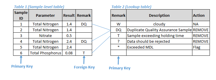
Figure 1. Example of relational tables with primary and foreign keys.
Review data dictionaries and field names before combining data from multiple sources into a spreadsheet or database format—do not assume that field names are equivalent between different data sources or even within a single data source. Even if the data dictionaries and field names are the same, data from different sources sometimes use different field and/or laboratory methods—consult a specialist as needed (e.g., chemist, taxonomist). A standard file structure and file-naming convention can improve version control management. Label files with unique identifiers such as dates or other indicators of version control. Multiple-gigabyte file sizes are increasingly common, especially with remote sensing imagery, spatial data, and large databases. Consider the storage and backup requirements of these large files. For example, you might need a separate server to accommodate the data needs for a project. If you are working with multiple people, also consider the implications of file storage choices for file transfer. Sample-level water quality data often are stored in a vertical format with a column for parameter or characteristic name and a column for result value, as shown in Figure 2. After data transformation, but before statistical analysis, it is often more convenient and space-efficient to convert the data to a horizontal format in which each parameter of interest has its own column where results for that parameter are reported. This approach allows for simpler identification of paired sampling data for multiple parameters (i.e., samples taken from the same station-date-time), which in turn makes identifying relationships among parameters possible.
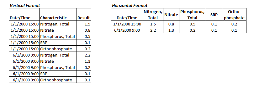
Figure 2. Examples of water quality data in vertical format (left) and horizontal format (right).
Effective data organization can improve the efficiency with which data can be checked for errors, cleaned, transformed, and documented. Sorting by location, source, parameter, or other column allows error-checking and transformation to be automated, which improves not only efficiency but also QA. Biological metric calculations typically are performed in spreadsheets or relational databases with embedded queries. To ensure that resulting calculations are correct and provide the intended metric values, a subset should be independently recalculated. One approach is to calculate (1) one metric across all samples, followed by (2) all metrics for one sample. When recalculated values differ from the values in the output matrix, reasons for the disagreement are determined and corrections are made. Reports on performance include the total number of reduced values as a percentage of the total, how many errors were found in the queries, and specific documentation of the corrective actions. A well-organized and functional database allows the index to be disaggregated to enable individual metrics and even taxa to be evaluated by biologists to help identify those having the most influence on an assessment.
Geospatial Information
A geographic information system (GIS) is a georeferenced database that has a geographic component (i.e., spatial platform) in the user interface. Spatial platforms associated with a database allow geographic display of sets of sorted data and make mapping easier. This type of databases with a spatial platform is becoming more common. The system is based on the premise that “a picture is worth a thousand words” and that most data can be related to a map or other easily understood graphic. GIS platforms frequently are used to integrate spatial data with monitoring data for watershed analysis. Spatial data such as shapefiles and model input files often are composed of a family of files that must be stored together to function properly. When transferring spatial data, keep in mind that all of the files must be transferred together and that project files such as MXD files must be relinked after the files have been moved. Geodatabases also are available, and they are becoming more common for storing multiple spatial data sets for a project while maintaining data set relationships, behaviors, annotations, and metadata. Spatial data should have metadata that include descriptive information about the data such as source, dates, processing, datum, and coordinate system. For any spatial data developed as part of an analysis, adhere to metadata standards such as those established by the Federal Geographic Data Committee. All spatial data should have the same coordinate system for comparison; therefore, transformations are often necessary. Coordinate systems include both a geodetic datum and a projection type. A geodetic datum describes the model that was used to match the location of features on the Earth’s surface to coordinates on the map. Common datums include the World Geodetic System 1984 (WGS84) for a good representation of the world as a whole and the North American Datum 1983 (NAD83) or 1927 (NAD27) for a representation of North America. A projection type is a visual representation of the Earth’s curved surface on a flat computer screen or paper (e.g., the Universal Transverse Mercator [UTM] or state plane). If available, a state plane coordinate system or other state system often is the most accurate system for a particular project area. Spatial data sets can exist in the same projection but be referenced to different datums and, therefore, have different coordinate values (e.g., latitude and longitude or UTM). To fully represent a location spatially and avoid errors or confusion, you need coordinates with the datum. Significant errors can be introduced when data with different or unknown datums are introduced, including errors in distance or area measurement and in relating the spatial location of features between data sets. GIS software or mathematical algorithms allow for the conversion of spatial data from one coordinate system to another.
Data Review and Cleanup
Data Review
Evaluating older historical data sets is a common problem because data quality often is unknown. Knowledge of data quality also is problematic for long-term data repositories such as STORET and long-term state databases, where objectives, methods, and investigators might have changed many times over the years. The most reliable data tend to be those collected by a single agency using the same protocol for a limited number of years. Selecting data from particular agencies with known consistent sampling and analytical methods will reduce variability caused by unknown quality problems. Requesting data review for QA from the collecting agency will reduce uncertainty about data quality. Supporting documentation also should be examined to determine the consistency of sampling and analysis protocols. The amount of documentation associated with a particular source can vary widely. Documentation of the source, including metadata documented in project reports, validation reports, and any database information, should be maintained along with the data. Research into the origin and documentation of a data source might be necessary to properly evaluate the data source. Potential sources for this documentation might include the website for the agency or group that collected the data, published reports, research articles, and personal communication with the original researcher or monitoring group staff. Consider this series of general questions when evaluating the quality of any data source and the applicability of the data to the current project:
- What was the original purpose for which the data were collected?
- What kind of data are they, and when and how were they collected?
- What cleaning and/or recording procedures have been applied to the data?
When evaluating a water quality data source, also consider the following questions, which are more specific to water quality data:
- Were the data generated under an approved QA project plan or other documented sampling procedure?
- If multiple data sets are being combined, were the data sets generated using comparable sampling or analytical methods?
- Were the analytical methods (detection limits [DLs]) sensitive enough to meet project needs?
- Is the sampling method indicated (e.g., grab, composite, calculated)?
- Was the sampling effort representative of the waterbodies of interest in a random way, or could bias have been introduced by targeted sampling?
- Are the data qualified? Are sampling and laboratory qualification codes or comments included? Are the qualification codes defined?
- Is sufficient metadata available about variables like sampling station location, date, time, depth, rainfall, or other confounding variables?
Be sure to document the rationale for including or excluding data from an analysis to ensure the transparency and defensibility of the decision-making process. Factors to consider when evaluating a data set include the accuracy, precision, representativeness, and comparability of the data set. Depending on the data use, different quality evaluation criteria might be needed to establish the best balance between data quality and usefulness of the data. An indication of the quality of the data used in the analysis should be included in project documentation and applied across all sources. Also, examine the data, looking for records that indicate that sample integrity was maintained, approved sample collection and analysis methods were used, established QC measures were in place for the laboratory conducting analyses, and instruments were calibrated and verified for performance. Documentation of evaluation criteria for each parameter is especially important when using data across multiple sources. Data might have been recorded using analytical methods under separate synonymous names or incorrectly entered when data were first added to the database. Review of recorded data and analytical methods recorded by knowledgeable personnel is necessary to correct these problems. To compare data collected under different sampling programs or by different agencies, sampling protocols, and analytical methods must demonstrate comparable data. The most efficient way to produce comparable data is to use sampling designs and analytical methods that are widely used and accepted such as Standard Methods for the Examination of Water and Wastewater (Rice et al. 2012) and EPA methods manuals. As stated earlier, if the impact of combining data is unknown or cannot be determined, then it might be appropriate to perform separate analyses on each source of data. The results of the separate analyses can then inform criteria development in a post-hoc analysis. To the extent practical, use multimetric indices (MMIs) of biological condition that have been regionally calibrated based on broader data sets of known quality. Using MMIs previously established by local, state, or regional agencies requires that the same or similar methods be used for field sampling and laboratory processing for other streams and sites being evaluated relative to best management practices or other issues. This approach of using accepted protocols and calibrated metrics and indices, coupled with sufficient and appropriate QC checks, improves defensibility of assessment results and increases confidence in natural resource management decision-making.
Data Cleanup
Before any further data processing occurs, consider initial data reduction to save time and effort. For successful data reduction, you must have a clear idea of the analysis to be performed and a clear definition of the sample unit to be used in the analysis. Data reduction may be an iterative process; a conservative approach of including more data may be more efficient than having to add data back into your analysis at later stages. Include these steps in reducing data:
- Select the long-term time period for analysis.
- Select an index period.
- Select relevant variables of interest.
- Identify the quality of analytical methods.
- Identify the quality of the data recorded.
- Estimate values for analysis (i.e., mean, median, minimum, maximum) based on the reduction selected
Reducing water quality data by screening nontarget data involves interpreting certain fields to select the data of interest to the analysis. Examples include:
-
- Sample media (e.g., water, soil, groundwater).
- Sample type (e.g., routine samples versus duplicate or QC samples such as spike samples, field replicates, or laboratory replicates). Checking routine values against duplicate values can be an effective QC check, but verify that duplicate values are not included in the data set used for analysis.
- Sampling type or location (e.g., effluent, ambient, stormwater, baseflow, pipes, finished water, or process water, are sometimes available). Sampling focused on effluent outfalls or pristine waters could bias a sampling effort. Sampling type or location can be an important indicator of sampling bias or spatial bias inherent in the data set resulting from opportunistic sampling rather than random sampling.
- Waterbody type (e.g., stream/river, lake/reservoir, estuary, ocean, wetland, canal, stormwater). You can use this field to further refine sampling data to the data of interest.
Data cleaning includes data checking and error detection, data validation, and error correction. This section describes typical efforts to standardize a data set created by combining multiple data sets and to screen a data set in preparation of analysis.
Standardization
Frequently, parameter names, comment fields, and result values are inconsistent across data sources or even within a single source. To combine data while retaining the original data, it is good practice to create user-specified fields to represent common parameters, standardized comments, and comparable values. Creating these fields enables you to correct errors and perform transformation while retaining the original data in separate fields as well as the capability to go back to the original data if necessary. Maintaining documentation of data transformation and error correction is especially important when the processes are being performed by anyone other than the primary data collector. Creating user-specified fields provides an opportunity to convert units to like units, standardize parameter names, interpret comment fields, convert nondetect values, or institute other data transformations. For instance, a user-specified data qualifier field might be used to flag or exclude blank samples or samples with nonnumeric characters in the value field. Figure 3 provides an example of how user-specified fields might be used to convert field names and units and to interpret comment fields. Another important application of user-specified fields is creating a column that documents the original source and the row identifier of the original source when merging data, so that if systemic issues are found in a source, they can be resolved and cleaned more effectively.
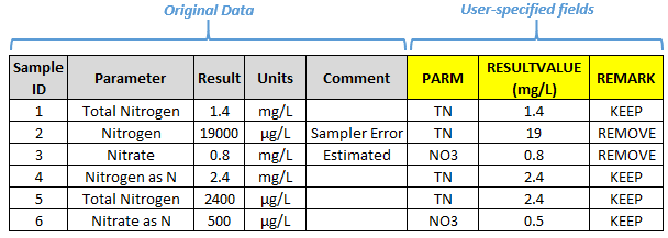
Figure 3. Example of user-specified fields.
Descriptive fields such as temporal indicators (e.g., date, year, time), sample depth, latitude/longitude, and units often are included in varying formats. Common fields and transformations that you should consider are described:
- Temporal fields: Ensures that all date and time fields are in the same format (e.g., DD-MM-YYYY, YYYY-MM-DD). It is recommended that you use military time and account for time zones. It might be helpful to have one field with “Date” and separate fields for “Year,” “Month,” “Day,” and “Time.” If a measurement of diurnal fluctuations is not needed in a parameter, averaging data by day might remove some inconsistencies resulting from data without time information or with slightly different times resulting from different labs processing the data or from data entry error. Searching for dates outside the range of interest or outside reasonable date or time values (e.g., month 12, day 31, year < 1900, time 24) can be a helpful screening tool. Having a sampling date is a reasonable minimum requirement for data.
- Depth fields: Depth should generally be a numeric field. Sometimes a surface or bottom indicator is included as well as a numeric depth field (e.g., S, B). It can be helpful, especially in lakes and estuaries, to add a separate text depth column for profile data that indicate surface, depth, or bottom measurements for some parameters (e.g., DO). Depth units should be standardized to a consistent format (e.g., feet or meters). Having a sampling depth (numeric field or indicator) is a reasonable minimum requirement for lake and estuary data.
- Latitude/Longitude fields: Ensures that latitude and longitude are reported in a consistent format. Latitude and longitude units are most often reported in degrees, minutes, and seconds (DMS) (e.g., 39°59’56.055”N, 102°3’5.452”W), decimal degrees (DD) (e.g., 39.999012, -102.052062), or sometimes UTM coordinates (e.g., 17T 630084 4833438). These examples all are roughly from the same point on the border of Kansas, Nebraska, and Colorado. To convert from DMS to DD, use the following formula:
(degrees) + (minutes/60) + (seconds/3600) = decimal degrees
If values are missing, consider digitizing from GIS or geocoding from an address if one is provided. One of the most frequent errors is omitting the negative sign (-) in decimal degree coordinates from the southern or eastern hemispheres. If all the records are from North America, all the longitude values should include a negative sign. Consider spatial accuracy: With today’s standards, be wary of decimal degree data with less than six digits of precision accuracy or seconds reported with less than two digits of precision (although for larger waterbodies, less precision might be acceptable). A typical minimum data requirement for station-level data is that the station must have a latitude and longitude measurement as well as the reported datum. Look for extreme values: Latitude should never be outside the range of 90 to -90 degrees; longitude, 180 to -180.
- Units: Units should be standardized by parameter and among parameters. Check for systematic incorrect reporting of units when converting all values for a parameter to one unit of measurement. Note that laboratories often report results on a weight-per-weight basis, such as parts per million (ppm) or parts per billion (ppb). In water samples, 1 ppm is essentially equivalent to 1 milligram per liter (mg/L) and 1 ppb is equivalent to 1 microgram per liter (µg/L) unless concentrations are very high (> 7,000 mg/L). In addition, µg/L and milligrams per cubic meter (mg/m3) can be considered identical in water samples in most cases. Outliers for a parameter might be an indication that data are reported in varying units. While it is a common practice not to include units as a data field in a database (i.e., the units are inherently known to the data generator or are documented in metadata), it is important to ensure that all units are identified.
Water Quality Characteristic Nomenclature
The naming conventions for water quality monitoring parameters often are inconsistent across different sources or even within the same source. Each separate analytical method should yield a unique variable (e.g., five ways of measuring TP results in five unique variables). Data generated using different analytical methods should not be combined in data analyses because methods differ in accuracy, precision, and DLs. Data analyses should concentrate on a single analytical method for each parameter of interest. Data generated from one method might be too limited, making it important to select the most frequently used analytical methods in the database. Data generated using the same analytical methods might not always be obvious because of synonymous names or analytical methods. Consistency in taxonomic conventions and indicator measurements also is important for biological variables and MMI comparisons. Review of recorded data and analytical methods by knowledgeable personnel is important to ensure that no problems occur with data sets developed from a particular database. One way to compare and combine data without applying a consistent naming convention is to add another user-specified name column to combine parameters under a unique name. Metadata from the data source, other fields within the data, and best professional judgment can be used to inform the consolidation of characteristic names into fewer unique parameters. Consult a chemist or the data owner if you are uncertain about what is being measured. If you still have questions about what parameter actually was being monitored, consider contacting the original monitoring group for clarification. Document the process of cross-walking the original parameter names to standardized parameter names. Using a lookup table to translate the fields often is an easy way to consolidate names and document the process in a transparent way. Keep in mind that categorizing data can lead to a loss of data and a potential reduction in quality. Storing data with the original resolution and exporting data as categorized for a particular use is good practice. Many monitoring groups also have parameter codes associated with each characteristic name. These codes provide a more detailed description of the parameter such as sampling method, analytical method, typical units, and sampling media. For example, USGS and the U.S. Environmental Protection Agency (EPA) have parameter codes associated with each parameter name (USGS NWIS EXIT; EPA Legacy STORET EXIT). In addition, EPA maintains a Substance Registry System (SRS) that provides a common basis for the identification of chemicals and biological organisms. The SRS pulls information from several registries, including Chemical Abstracts Service (CAS) number, taxonomic serial number (TSN), and EPA internal tracking number (EPA ID number). A CAS number or CAS registry number (CASRN) is a unique number assigned by CAS to chemical substances, and additional information about each substance is maintained along with the CAS number. A TSN is a unique numeric identifier used to identify biological species. Routine biological monitoring programs in the United States typically collect data on benthic macroinvertebrates, fish, and algae; some programs include macrophytes, seagrasses, corals, or reptiles and amphibians. Biological data often are reported with varying levels of processing—from raw species observations and operational taxonomic unit abundances to algal biomass (e.g., AFDM or chlorophyll a) and biological metrics (e.g., algal, invertebrate, fish). Metadata are vital to documenting the collection method, sample identification process, index calculation method, and other attributes of the data. All biological sample data in a table should be based on the same collection method, processing, subsampling, and taxonomy. To avoid confusion, use a completely separate table for data collected using different methods.
Biological Data Nomenclature
Naming conventions for species identified in biological assessment data often follow different formats. This section presents an overview of the species identification process and naming conventions. Depending on the organism, several options for unique identification might be most applicable.
- The Integrated Taxonomic Information System (ITIS) EXIT uses the TSN to provide a list of unique biological species, with more information about each species available.
- American Fisheries Society Fish Identification guidance: Common and Scientific Names of Fishes of the United States, Canada, and Mexico (Nelson et al. 2004).
- The Academy of Natural Sciences of Drexel University has a series of online databases and collections Exit for species identification.
- Taxon names: EPA’s SRS and USGS maintain acceptable lists of taxon names that can be used as a basis for unique identification:
- EPA SRS
- Catalogue of Life Exit
- Global Biodiversity Information Facility (GBIF) Name Parser Exit
A unique taxon name should be identified, but often identification is made down to only the family or genus, not all the way to the species level. Increasingly, genetic signature data such as DNA barcodes might be included. Depending on the use of the data, identification to the genus level or higher might be acceptable for metric calculations or other uses. Genus-level taxonomy is the principal hierarchical level used by most routine biological monitoring programs for benthic macroinvertebrates, although occasionally the family-level is used. Be aware that, in some cases, unresolved taxonomic issues might be present such as data with no parent family and daughter genus data in the same data set. Taxonomic classifications are opinions, and differing opinions by different taxonomic experts can lead to the same organism being classified differently. Databases should have the flexibility to include alternative names to capture disagreement in taxonomic opinion as well as different accepted names (Chapman 2005a). Some databases store taxon names in one field, which can lead to more errors. It is recommended that taxon fields be divided into separate fields (e.g., genus, species, infraspecific name, certainty) to improve QA and organizational capabilities. Plants especially have several levels below species that are frequently used—subspecies, variety, subvariety, forma, subforma, cultivars, and hybrids. Misspellings are common in scientific names. Finding spelling errors using one of the sources mentioned above should be straightforward at the family or genus level but might be difficult at the species level. Similarity algorithms can be used to compare and determine the degree of similarity between scientific names to identify misspelling errors. Table 1 provides some typical examples of misspellings for just one species (Karenia brevis, or red tide) (e.g., Dinophycae, Karania, brev); lack of consistency in data entry (e.g., brevis?, sp. brevis, aff. brevis); and changes in naming convention (e.g., K. brevis was formerly called G. breve or P. brevis).
Table 1. Examples of differences and errors in taxon naming convention
| Class | Genus | Species |
|---|---|---|
| Dinophyceae | Karenia | brevis |
| Dinophyceae | Karenia | brevis? |
| Dinophyceae | Karenia | aff. brevis |
| Dinophyceae | Karenia | sp. brevis |
| Dinophyceae | Karenia | brevis |
| Dinophyceae | Karenia brevis | |
| Dinophyceae | Gymnodinium | breve |
| Dinophyceae | Ptychodiscus | brevis |
Screening
Data screening is an important processing step in preparing a data set for analysis. Screening can include identifying and accounting for duplicate or missing data, especially large or small values (outliers) and data re-marked with qualifier text or codes for duality control concerns as well as some other considerations specific to biological data.
Duplication and Missing Data
Duplication frequently occurs in water quality data sets. It might be the result of obtaining the same data from different sources or simply data entry error. Duplication can occur within a single data source or among different data sources. Merging two data sets sometimes creates new inconsistencies and duplication. Because duplication can skew and bias data, instances should be flagged and screened from the analysis as much as possible. Some samples might resemble duplicate entries but actually have different depths, times, or other distinguishing features. If the only fields that are different are descriptive fields, such as comment fields, that might indicate duplication. The organization identifier and sampling name can be good indicators that duplication has occurred, but also look for duplicate values in the data over the same time frame. For example, several identical numerical values on the same day might indicate duplicate data. Sorting the date chronologically and looking for duplicate sample results is one way to begin to identify duplication. MS Excel has features you can use to identify and highlight duplicate values in a field; when the data are sorted chronologically, Excel can identify potential duplicates. Duplicate records should be flagged using a user-specified field but generally not deleted. Simply deleting duplicate data, rather than flagging and excluding the data, creates a potential for error and data loss that is difficult to identify. Blank fields should be checked to determine whether the value was intentionally left blank or is the result of an error. It is good practice to document the reason for a blank value in a separate field (such as “not applicable”, “not relevant”, or “unknown”), but reasons are not always well documented. A user-specified data qualifier field might be used to flag or exclude blank samples. The data should be 100 percent error-checked for transposition errors and typos. Screen the data for inappropriate nonnumeric characters. The reality of any monitoring program is that samples will be missed, equipment will fail or be overwhelmed, droughts and floods will occur, and sample analysis limitations will be exposed, resulting in missing values (USEPA 2016c, p. 7-20). Data missing randomly generally has a minimal effect on estimated relationships, but data missing in a predictable pattern can bias them and should be considered further. For example, data often can be missing as the result of systematic issues encountered during data collection such as instrument DLs. You can statistically test for a particular variable to determine whether it is missing at random by splitting the data set into one subset in which the variable has a value and a second subset in which a value for the variable is missing. Then, you can examine other measured variables for significant differences across the two subsets. If data are missing at random, then samples with missing data can simply be excluded from the data set. If data are not missing at random, then analysts should consider the effect of the missing data. When a data set includes a large number of missing values, it might be necessary to consult a statistician about the most appropriate method either to develop a complete data set or to apply appropriate modeling approaches that can use incomplete data.
Outliers
Outliers are especially large or small sample values relative to the distribution of the rest of the data. Outliers are of concern because they might misrepresent the distribution and can have a strong bias on average values and nutrient-biological response relationships. Potential outliers can be initially identified using exploratory data analysis methods such as summary statistics, histograms, normal-quantile plots, and scatterplots . Plotting the data in a time series plot by date or stratifying by season or flow conditions can reveal patterns in extreme values that might be related to an actual event or measurement or recording error. Several statistical tests to confirm that values are true outliers also are available that include Dixon’s Extreme Value Test, the Discordance Test, Rosner’s Test, and Walsh’s Test (refer to USEPA 2006 for guidance on performing these tests). Several software programs for identifying outliers of geographic coordinates are available that include spOUTLIER and Diva-GIS (Chapman 2005b). Ultimately, the decision to correct an outlier, remove the value from the data set, or use the data point should be based on best professional judgment and have a scientific basis supported by visual analysis and/or a statistical test. Both failure to identify true outliers and removing false outliers will result in distortion of the statistical analyses of the data. Removal of outliers should focus on cases in which the cause can be identified as measurement or equipment error, laboratory error, or recording error (USEPA 2016c). Environmental data often contain legitimate extreme values, so correct or remove outliers with caution. Initial screening of data often is a necessary step before outlier analysis is performed. Sometimes data entry software requires that analysts add an entry, so dummy values such as ‘0’, ’-99’, ‘Null’, or ‘NoData’ are entered. Analysts should evaluate and address zero or negative values for most variables unless there is a legitimate reason for those variables to have a zero value (e.g., temperature). A table of minimum and maximum values can be used to identify and potentially screen out negative or extreme values as a first-step screening tool. Note that the screening values differ by parameter; depending on the sampling, different ranges of values should be expected for different parameters. Environmental data often contain legitimate extreme values, so correct or remove outliers with caution.
Data Qualifiers
Data qualifiers—codes or notations that provide additional qualifying information about the measurement value being reported—should be included in a water quality data set. A data set that does not include data qualifiers could be a red flag about the quality of the data. Contact the monitoring group for clarification if possible. Qualifiers can take a variety of forms depending on the data set, including a system of qualifier codes or flags, entries in comment fields (sampling and/or laboratory), and fields for type of sample (e.g., duplicate, spiked, replicate, routine). Analysts will need to interpret data qualifiers to be able to use them to screen out data with quality concerns. It is not recommended that samples be deleted at this stage, but flagged for exclusion from the analysis after all applicable data qualifiers have been interpreted. If samples are excluded from analysis, reasons for exclusion should be documented. Creating an internal, user-specified qualifier field can be useful for documenting choices and combining multiple data qualifier fields into one field for decision-making. While there are several commonly used sets of data qualifiers, there is neither a universal set that applies to all types of analyses nor a universal specification for their use. Table 2 provides some examples of data qualifiers. Data qualifiers can provide descriptive information about a sample without calling data quality into question (Group 1), provide an indication of how censored data were reported (Group 2), or call into question the quality of the data (Group 3). Samples with qualifier codes in Group 2 will need to be further processed (refer to Censored Data for further guidance). Qualifiers such as those in Group 3 could possibly lead to sample screening. Check the metadata or other documentation associated with a data set for the key and description of each qualifier code specific to the data set.
Table 2. Examples of data qualifiers (codes and descriptions)
| Group 1 – Descriptive | |
|---|---|
| A | Reported value is the arithmetic mean (average) of two or more determinations. |
| D | Measurement was made in the field (i.e., in situ). |
| F | When reporting species, F indicates the female sex. |
| AP | Approved for publication; processing and review completed. |
| Group 2 – Censoring | |
| U, ND | The compound was analyzed for but not detected. Value is less than the method detection limit (MDL). |
| I | Reported value is greater than or equal to the laboratory MDL but less than the laboratory practical quantitation limit. |
| T | Reported value is less than the laboratory MDL. It is reported for informational purposes only and shall not be used in statistical analysis. |
| M | Reported value shall be the laboratory practical quantitation limit. This code shall be used if the level is too low to permit accurate quantification, but the estimated concentration is greater than or equal to the MDL. |
| Group 3 – Data quality in question | |
| 8192 | Sample lost in lab; not analyzed. |
| 512 | Labeling error; sample identifier uncertain or unidentifiable or sample identifier is inconsistent with analytical results. |
| 16 | Deviation from standard method. Result is probably okay. |
| E, J | Value was computed from estimated unit values. Where possible, the organization shall report whether the actual value is estimated to be less than or greater than the reported value. |
| < | Value is known to be less than the reported value. |
| > | Value is known to be greater than the reported value. |
| Q | Sample held beyond the accepted holding time. |
| P | Provisional data subject to revision. |
| K | Value is affected by instrument calibration drift. |
| R | Significant rain in the past 48 hours. |
| X | Value is erroneous. It will not be used. |
| ? | RData are rejected and should not be used. Some or all of the QC data for the analyte were outside criteria, and the presence or absence of the analyte cannot be determined from the data. |
| & | Value is affected by unspecified reasons. |
Sources: Florida DEP IWR; USGS NWIS EXIT; USGS Upper Midwest Environmental Sciences Center EXIT; ANERR—Alabama NERR data.
Biological Data-Specific Considerations
Some screening considerations are unique to biological or habitat data. All calculated metrics should be correct for the appropriate bioregion or biological class; scored values should be provided. Seasonal community changes such as differences in taxa reproduction, growth, and emergence phenologies can affect the comparability of calculated metrics. Observations should be plotted by month to determine whether significant seasonal bias is present in the sampling data. If the data are simply metrics, they can be reported in the same table, using different codes for the same metric collected two different ways (e.g., EPTRichness_HesterDendy, EPTRichness_Sweep). The data should be evaluated for collection method compatibility and excluded if methods are not found to be compatible. Alternatively, the data is evaluated independently and considered as multiple lines of evidence for the purposes of nutrient criteria development. Similar to water quality data, biological assessment data often include a series of data qualifier codes or comment fields that further describe the data. These fields might include life stage codes, organism condition codes, missed level reason codes, or other general notes. The degree of certainty of the taxonomic identification should be included. Many of the QC techniques described in previous sections also apply to biological data (e.g., duplicate screening, outliers, source documentation, spatial data analyses). An example of a QC technique with biological data is described in the Virginia Ecological Limits of Hydrologic Alteration (ELOHA) report (USEPA 2012b). Multiple sources of fish and benthos data were compiled for analysis for this project, and one QC check was to plot sample abundance across data sources. Figure 4 shows sample abundance by data source for benthos. It was determined that the USGS NAWQA benthos results were reported as densities by taxon rather than sample counts as with the other sources. The NAWQA density values included multipliers to account for subsampling and area sampled, but the multipliers were not reported along with the data set. The study analysts contacted USGS and received the multipliers, which allowed the analysts to convert the data back to counts per sample to make the data comparable to the other data sources.
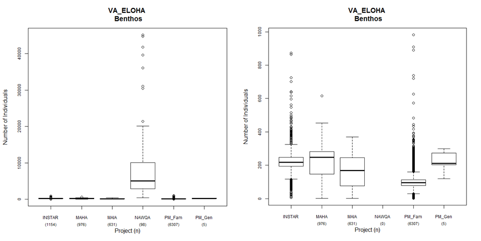
Figure 4. Benthos sample abundance by data source from the VA ELOHA project with the NAWQA data source (left) and without the NAWQA data source (right) (USEPA 2012a).
Censored Data
Data reported as not detected or below a DL should be used but accounted for statistically (Bolks et al. 2014).
Censored data are data that are measured to be less than or greater than a DL or quantitation limit (QL). DLs, such as a method detection limit (MDL) or instrument detection limit, are the lowest concentration that can be distinguished from a zero value (i.e., the parameter is present, but it cannot be quantified). QLs, such as the practical quantitation limit (PQL), represent the lowest concentration that can be not only detected, but also quantified with a degree of precision. Laboratories often set and report a PQL associated with each testing method performed at that laboratory; thus PQLs vary from laboratory to laboratory. MDLs also vary based on the method of collection, storage, and analysis of a particular parameter. Each combination of parameter, analytical method, and laboratory should have its own DL and QL reported along with each censored data point. When data are described as nondetect or left-censored (ND, U, <), the actual value of the data lies somewhere between zero and the DL. Interval-censored values lie between the DL and QL. Right-censored (>) data report values greater than a high-end QL, such as too numerous to count in bacteriological analyses, flow exceeding flow gauge limits during floods, or Secchi depth measurements of visible on bottom. Table 3 provides descriptions of the types of censored data.
Table 3. Common descriptions or terms associated with different types of censored data
| Left-censored | Interval-censored | Uncensored | Right-censored | |
|---|---|---|---|---|
| Description |
|
|
|
|
Source: Bolks et al. 2014. Censored data are of particular concern with water quality data because of varying treatment and reporting of nondetected values. It is common for nondetects to be reported with DLs omitted, DL types undefined, zero entered as the reported value, a value less than the DL reported, or “less than a value” (e.g., < 0.05) entered as the reported value. Varying approaches to handling censored data will need to be standardized in any analysis using multiple data sets. There are a variety of methods for processing censored data, and approaches vary depending on the data and purpose of the analysis. Documentation of how censored data are processed is a crucial part of any analysis. Extensive research in water resources as well as in other fields of science such as survival analysis (e.g., how long does a cancer patient live after treatment) has been conducted into numerous techniques of accounting for censored data. One deficiency over the last 20 years has been the lack of readily available tools for widespread use, making many of the tools out of reach for general use. Efforts to improve the availability of these tools is continuing. With improved tool access, past methods for accommodating censored observations can be avoided. The most notable method is simple substitution, which involves the replacement of censored observations with zero, ½DL, or DL. Although simple substitution is commonly used (and even recommended) in some state and federal government reports as well as in some refereed journal articles, there is no real theoretical justification for the procedure. Substitution can perform poorly compared to other more statistically robust procedures, especially when censored data represent a high proportion of the entire data set. More egregiously, some reports have simply deleted observations less than the DL. In the past, some researchers have recommended simply reporting the actual measured concentrations even if they are below the DL. This approach has not become popular as laboratories are reluctant to implement such a practice, although Porter et al. (1988) suggested that an estimate of the observation error could be reported to better qualify the measurement. While simple substitution might be convenient for initial exploratory analyses using spreadsheet tools, more robust procedures are available and are recommended. If substitution of numerical values for nondetects is believed to have a significant effect on the results of an analysis, a sensitivity analysis can be performed. This method can be performed by substituting all zeros or the full DL or QL for nondetects, instead of the current substitution method, and repeating the results to determine whether the analysis is sensitive to the selected substitution method. In addition to substitution or replacement, other more statistically robust imputation procedures are available for processing censored data. These techniques are especially applicable in cases in which more than 10–15 percent of the data are nondetects and a sensitivity analysis shows the data to be sensitive to the substitution method. Cohen’s method provides estimates of the mean and standard deviation that account for nondetected data, but it does not provide replacement values for each nondetect value (USEPA 2006). In addition, the statistical software package R offers several methods for estimating summary statistics from censored data such as maximum likelihood estimation, robust regression on order statistics (robust ROS), and the Kaplan-Meier method. A test of proportions might be appropriate in cases in which more than 50 percent of the data are below the DL but at least 10 percent are detected. Rather than reporting mean values, a percentile of the data greater than the DL could be reported (e.g., hypothesis test of the 75th percentile or simply 95 percent of the TN data are below a threshold).