Run Decision Support Scenarios

After you set up the model, you can run scenarios at different nutrient concentrations. The goal is to change the levels of nutrients entering the system until a previously determined  is met, then to determine the level of nutrients in the water body that corresponds to attainment of the target and designated use support. Targets should be selected based on available data, scientific defensibility, and sensitivity to nutrients. Potential targets include historic seagrass colonization depths and locations (water clarity), phytoplankton biomass (chlorophyll a), and protection of sensitive faunal communities (DO). Ideally, your stakeholders or you should select the most appropriate targets and endpoints prior to beginning model development.

You might begin with evaluating the calibrated model scenario to determine if the endpoints are attained.

• If your endpoints are attained, you can evaluate how much additional nutrient loads can enter the water body while continuing to attain the endpoints.
• If your endpoints are not attained, you need to evaluate nutrient reduction scenarios.

In the case of reduction scenarios in an estuary, you reduce watershed anthropogenic nutrient loads from calibrated levels until the assessment endpoints are met. Since lakes and estuaries can receive discharges from more than one tributary stream, modelers need to determine a method of distributing the reductions among these tributaries.  One way is to distribute the reductions in proportion to the estimate of natural and anthropogenic loading. For example, if you estimate the aggregate protective loading to the water body as a 10 percent reduction in loading from anthropogenic sources, the loading distributed to each terminal reach would be based on 100 percent of the natural loading (i.e., no reduction) from each tributary and a 10 percent reduction in the anthropogenic loading from each tributary. The natural loading can be estimated with a watershed model such as HSPF or LSPC by simulating non-anthropogenic conditions in which all point sources of nutrients are set to zero and nonpoint sources of nutrients are set to forest or wetland land use levels. Since the non-anthropogenic proportion of load from a watershed changes daily, it might be necessary to calculate the reduction for each day of the time series data set. You then can enter the resulting daily flows and reduced concentrations into the hydrodynamic and water quality models. This method of reducing nutrients in proportion to the anthropogenic load contributed by each stream maintains the natural, background nutrient levels while reducing the controllable, anthropogenic part of the nutrient load. This approach has been used in estuaries, rivers, and lakes. EPA’s Methods and Approaches for Deriving Numeric Criteria for Nitrogen/Phosphorus Pollution in Florida’s Estuaries, Coastal Waters, and Southern Inland Flowing Waters discusses several methods of distributing reductions (USEPA 2010a).

Another method you could use would be to simply reduce all model boundary conditions by the same percentage and focus on the nutrient responses in the main water body. By paying attention to the source of loadings, i.e. point sources or specific landuses, however, you could obtain a more realistic prediction of expected management actions and develop criteria that are more relevant to those actions. This is true because the timing and location of loadings is important.

For steady-state, critical condition modeling, you might consider other loading strategies. Some states define critical design conditions in their rules such as setting all inflows to minimum 7-day average flow with a 10-year return period, a critical temperature, or certain DO and BOD. A more realistic condition is to base critical conditions on monitoring data collected during low-flow events, then—while holding tributary inflows constant—increase or decrease loadings to attain the targets.

Evaluate Model Results and Compute Criteria (Chlorophyll a, TN, and TP)

Evaluating model results involves comparing the results to the targets developed previously when the conceptual model and ecological endpoints were determined. Targets can be expressed as a single value for the water body or as a set of values that vary over space (e.g., water body segment) and time (e.g., season). The model output might be much more detailed in space and time than the targets. Consequently, you might need to aggregate the model output into data that are comparable to the targets. In addition to comparing the magnitudes of results to the targets, you will need to consider the frequency with which the target should be met to support the designated uses.

Once you have determined that the target is attained at the proper frequency, time-scale, and space-scale, you will be ready to calculate the criteria. You will compute the criteria based on the model results; however, you have many options such as setting criteria equal to the maximum, median, or average concentration.

Evaluate model results and post-process output and compute metrics

Comparing model predictions to the ecological endpoints and targets might require aggregating the data over time and over horizontal or vertical model cells or across multiple reaches. Evaluating model results can be an iterative process in which different averaging strategies are tested and targets are revised. Before continuing, consider comparing how modeling for criteria development is different from TMDL and permit modeling.

There is a distinction between applying models to develop numeric nutrient criteria and applying them to develop TMDLs or permit limitations. Because criteria development involves defining ecological endpoints and targets as well as evaluating whether they are met adequately to protect the uses, there is more flexibility in interpreting model results in that process than in developing a TMDL or permit limit. The objective in developing criteria is to define and meet the model targets that represent the ecological relevant endpoints (and protect the designated use). The presumption is that numeric targets do not exist and are a part of the modeling analysis. In contrast, when developing a TMDL or water quality-based effluent limit for a permit, one or more criteria exists and must be targeted. The existing criteria are written specifically to support the designated use, and attention must be given to making sure the criteria are met as intended. An exception to that rule is if the existing criteria are in narrative form instead of in numeric form. In that case, developing a TMDL becomes more similar to criteria development. Interpreting narrative criteria might require you to develop a conceptual model and ecological endpoints as you would in developing criteria.

Compute Criteria (Chlorophyll a, TN, and TP)

Nutrient criteria are specified as chlorophyll a, TN, and TP concentrations or loads not to be exceeded, which can be set for a growing season period, an annual period, or an annual period not to exceed more than a given frequency. Model results can be utilized to derive the concentrations and load criteria by averaging results over the zones, cells, or stream reaches of interest. Or, if criteria will be compared at a select station, results from the model at that specific location can be used. In some cases, such as in the 1 in 3 exceedance methodology, this will account for periods or years where natural conditions may be abnormal, causing higher concentrations and loads, such as hurricanes which may churn up bottom sediment in a lake or estuary and temporarily increase concentrations. In addition to setting the criteria for a lake or estuary water body, if a watershed model was used to derive loads entering the water body, protective criteria for the tributaries entering the water body can be calculated.

Using an annual average duration and one out of three frequencies as an example, we can derive criteria from the model results in one of two ways:

• Calculating the 90th percentile of the annual average concentration. Figure 7 shows the probability density function and cumulative probability function of a log-normal distribution. The 90th percentile of the normal distribution of annual average natural logarithms is used, which gives the log of the TN concentration of -0.90, which equals 0.406 mg/L (e^-0.9=0.406).
• Table 8 shows a way to calculate the modeled annual geometric mean that was exceeded only once in a 3-year period.
  • The second column is the annual geometric mean for each year.
  • The third column is the value exceeded only once in a 3-year period. The highest of the six values is the TN criteria, which would be expressed as an annual geometric mean of 0.33 mg/L not to be exceeded more than once in a 3-year period.

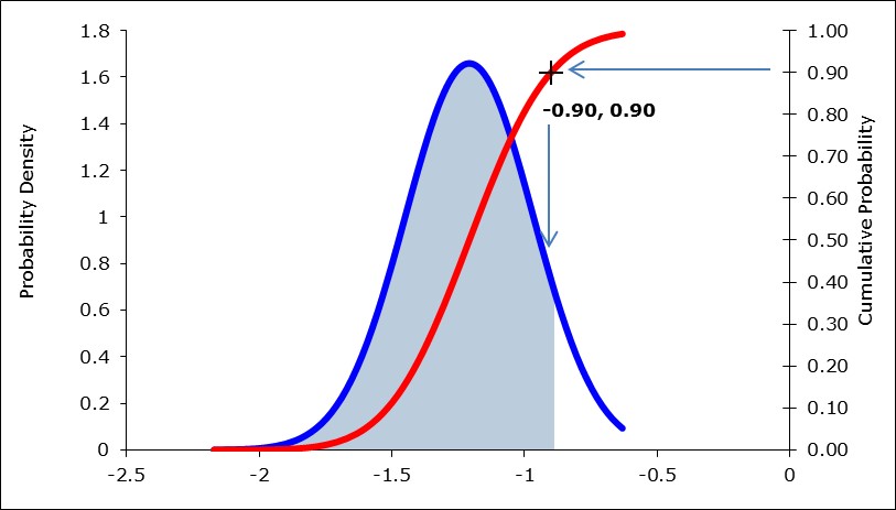
Figure 7. Calculate upper end of distribution of annual average of natural logarithms