
Configuration & Calibration
Configuring Spatial Extent and Resolution
When configuring a model, you must consider both spatial extent—the specific boundaries of the area to be assessed—and spatial scale—the size of reaches, segments, or grid cells to be provided in each dimension. Factors such as physical, chemical, and biological properties; applicable water quality standards; and monitoring data will influence the spatial design of your model.
The model’s extent should be large enough to cover at least the area of interest and extend beyond to boundaries that can be informed with data. Boundary data that describe the flows and water quality characteristics of the water entering a model must be input to the model. In general, the boundaries should be located beyond the influence of the waterbody area being evaluated and beyond the location for which model predictions are needed. Boundaries should be located where flow or stage and water quality are well monitored. Upstream boundaries should be located at a fall line, dam, or gaging station in riverine reaches. For a lake, typically the entire waterbody is modeled, from the upstream extend of ponded water to the dam. For larger lakes, such as the Great Lakes, smaller sections can be modeled, but the boundary must be far enough away from the area of interest to not impact the modeled results. For an estuary, if the segment of interest is a tidal river, the downstream boundaries could be located at the mouth of the estuary. In most systems, however, the preferred boundary is nearby in the open ocean. For a large estuary with relatively unaffected seaward reaches, the downstream boundary can be located within the estuary near a tidal gage and water quality monitoring station.
Water quality monitoring stations in the open ocean are not always available and, if that is the case, remote sensing data such as the National Aeronautics and Space Administration’s (NASA’s) SeaWiFS and MODis data might be helpful. For example, EPA processed the NASA OceanColor L3 SMI remote sensing data product to provide chlorophyll a concentration estimates for the Florida Big Bend Estuary model ocean boundary (Feldman and McClain 2013). Note, as is the case for other data sources, applicability of satellite data for calibration will be dependent on the quality of the data.
Another boundary data-related aspect for an estuary or lake model is whether to model the watershed draining to the water body. That decision depends on the data you have for the tributaries flowing into the estuary and the use of the model. A watershed model may be useful because it allows you to evaluate changes in loadings under historical (natural) land uses and future conditions or land uses. Otherwise, these loadings will have to be estimated using historical data, if available, and literature references. The nutrient and other constituent loads will likely be the largest influence on a receiving water. Some streams are monitored for flow and water quality, but others are not. Flows and water quality data from ungaged and unmonitored streams can be estimated by developing a watershed model for a larger area that is calibrated to a stream in the watershed with data. Another alternative is to estimate the flows and water quality using data from nearby streams that have been monitored.
Configuring based on water quality standards and physical, chemical, and biological differences
In addition to boundary data, it is also important to consider the spatial resolution needed to understand nutrient loading and response in the locations for which you want to derive criteria. For example, a model grid with large cells might be sufficient for deriving nutrient criteria in the main bay of an estuary, but not for the smaller bayous or tidal creeks. Additionally, the spatial resolution of a model must be able to represent details of water quality standards. For example, the Chesapeake Bay has five tidal water designated uses, each with specific water quality criteria, and a model should be configured to provide water quality predictions in each of the areas. The same consideration applies to lakes and reservoirs, where smaller embayments often exhibit different water quality than the main open water portion. Rivers and streams usually are broken into reaches of similar slope and physical characteristics. Many rivers and streams have shallow areas near the shores with deeper thalwegs. Benthic algae and macrophytes might grow in those shallow areas, but are absent in the deep center areas. With this in mind, consider whether this side-to-side lateral dimension can be represented as a single, well-mixed section or if the river should be modeled in different lateral segments. Similarly, consider if the river is stratified and whether you should model the vertical layers.
Monitoring data considerations in model configuration
Assessment programs use data collected at monitoring stations, which might be averaged over a water body. A model should be configured to produce meaningful output in the location that best represents the location of monitoring stations and methods. For example, if grab samples of DO are collected routinely at a depth of 5 feet, the modeler should consider that when selecting and configuring a model. A well-mixed river could be modeled with a 1-D model; however, a deep, stratified river would require a model that can distinguish the vertical profile. The vertical resolution should be configured so the 5-foot depth is well represented by one of the model layers. Similarly, if monitoring in a lake is sampled and assessed at distinct points, then the model should be well calibrated at those points. If the lake is divided into spatial zones, then the group of model cells representing each zone should be averaged.
Loadings from also must be entered into the model. You often can obtain the wastewater discharger location, flows, and water quality loads/concentrations from the EPA Permit Compliance System website. You also can request the data from states and municipalities. Depending on their permits, the wastewater dischargers might not be required to monitor all water quality constituents. In those cases, you will need to estimate the loads and concentrations, which can be done by referring to literature values and papers to determine the typical discharge concentrations for each facility type. In addition, depending on the level of model complexity, you could include loadings from land application systems (LAS) and/or septic systems. The spray rates, concentrations, and LAS area can be requested from the state and municipalities as well. Many states have publicly available data on the number and locations of septic systems. The percolate concentrations discharged from the septic systems and the associated attenuation factors can be determined using measured data if available. Otherwise, you will need to estimate this information using literature values.
Water withdrawals should be included in the model. Because of safety concerns, the location and withdrawal rate data are typically not publicly available and you will need to request them from the state prior to developing the model.
Model calibration and validation and estimating uncertainty
Before managers base decisions on model predictions, modelers need to demonstrate that a model is sufficiently configured and calibrated to accurately represent the system modeled. Calibration is an iterative process involving three exercises:
- Model calibration—evaluation of the degree to which a model corresponds to reality; involves comparing predicted results to observed data.
- Sensitivity analysis—assessment of the degree to which model predictions change in relation to perturbations in specific parameters or forcing variables/functions.
- Uncertainty analysis—assessment of sources of error and error propagation to model predictions; evaluation of confidence intervals for model predictions..
Model calibration is typically divided into hydrologic or hydrodynamic calibration, and water quality calibration. Modelers calibrate hydrologic or hydrodynamic processes first since the movement of the water affects the water quality processes. To determine when a model is well-calibrated, modelers commonly assess simulation error by comparing model results and observations. Modelers can do a spatial validation and compare results to data in a similar but different area of the model. Modelers also might perform validation by running the model for a different time period with environmental conditions substantially different from those during initial calibration and comparing those model results with observed conditions. The initial calibration results and validation results are compared to observed data sets with graphical plots and error statistics.
Graphical plots are used to aid calibration and include time series plots, cumulative frequency plots, and regression plots. Calibration can be demonstrated through visually inspecting time series plots of model results versus observed data as shown in Figure 3.
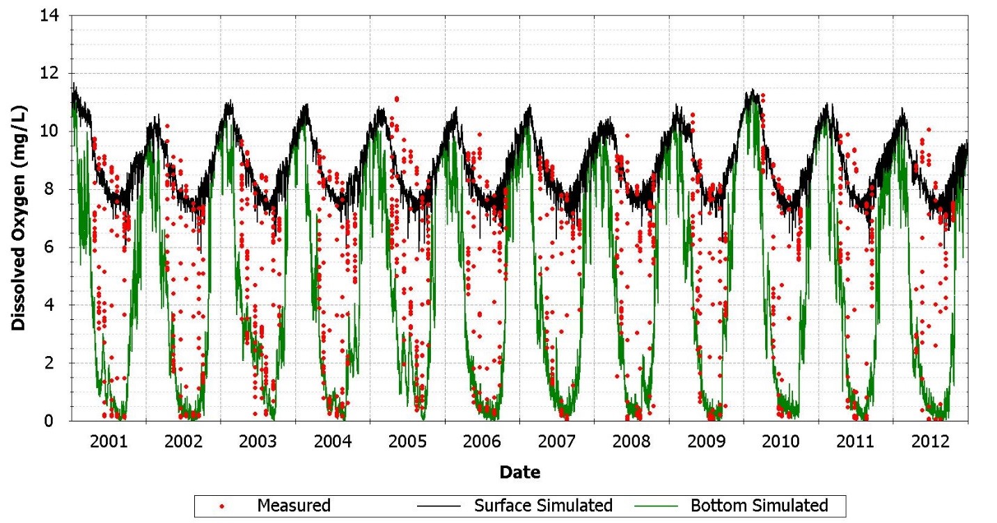
Figure 3. Timeseries Plot
Additionally, regression plots of modeled data versus observed data can be useful by showing how close the points plot to a 1:1 line and by comparing the slope and intercept of the linear regression to the 1:1 line, as shown in Figure 4.
-

Figure 4. Regression plot of TP (lbs/day) load scatter
Error statistics such as percent bias (PBIAS), relative error, average error, and root mean squared (RMS) error also are commonly used in calibration. These statistics judge the model’s precision by comparing modeled and observed values. Very few published, peer-reviewed papers address what constitutes a good calibration—consequently modelers, managers, and stakeholders should work together to determine what acceptable error is for their project. Defining a fixed set of standards for the quantitative calibration statistics can remove any subjectivity that might otherwise affect a good calibration. A degree of flexibility is recommended, however, because the model might not be able to match the observed data as well as desired.
Examples of Error
Data collected by agency is sometime rated to provide an indication of the data quality. Errors in data measurements, which can be introduced by sampling errors or laboratory errors, can impact the ability of the model to represent the measured values. For example, the USGS rates stream flow records as excellent, good, and fair with 95 percent of daily flow measurements within 5, 10, and 15 percent of the true value, respectively (Risley and Gannett 2006). Model error within that range of observed data error would be acceptable. Donigian (2002) lists general guidance on percent mean errors for hydrodynamic and water quality model results in Table 5.
Table 5: Calibration/validation targets or tolerances, annual and monthly results for HSPF applications (Donigian 2000 in Donigian 2002)
| % Difference Between Simulated and Recorded | |||
| Very Good | Good | Fair | |
| Hydrology/Flow | < 10 | 10 – 15 | 15 – 25 |
| Sediment | < 20 | 20 – 30 | 30 – 45 |
| Water Temperature | < 7 | 8 – 12 | 13 – 18 |
| Water Quality/Nutrients | < 15 | 15 – 25 | 25 – 35 |
| Pesticides/Toxics | < 20 | 20 – 30 | 30 – 40 |
Flynn et al. (2013) suggested an acceptable PBIAS of 10–28 percent for benthic algae based on the range in replicate sampling data. Error tabulated by Martin and McCutcheon (1999) for DO from several estuary models ranged from 5 percent to 56 percent for relative error and from -4 percent to -1 percent for average error.
Sensitivity analyses also are very informative in the calibration process. In sensitivity tests, multiple model simulations are run while one variable is perturbed. The model output is then analyzed to see how that variable impacted the model results. The process is repeated for the most important parameters or input variables. Sensitivity analyses are used during calibration to identify which parameters have the most influence on particular model results. The modeler can then focus on adjusting those parameters.
The third exercise in calibration is to estimate uncertainty of the model output. This error analysis involves estimating the uncertainty of each of the significant model parameters, initial conditions, and boundary conditions and determining the combined uncertainty in the output (Martin and McCutcheon 1999; Camacho et al. 2014). The process of quantifying uncertainty is often neglected, but is important so decision makers can include appropriate safety factors [see EPA’s Guidance on the Development, Evaluation, and Application of Environmental Models (2009) for more information]. Modelers and decision makers should determine the degree of uncertainty that is acceptable within the context of the specific model application and estimate the uncertainties underlying that model. For example, consider TN criteria: The uncertainty analysis can determine the size of the interval around the TN concentration predicted to support the designated uses. A wider interval might lead to a lower criterion being established to protect the designated uses.
Uncertainty analysis has always been a difficult task for mechanistic water quality modelers principally because of insufficient data to provide unique estimates of many of the model parameters (Reckhow and Chapra 1999, see also Camacho et al. 2014; Camacho et al. 2015). As a consequence, tabulations of suggested parameter values such as EPA’s Rates, Constants, and Kinetics Formulations in Surface Water Quality Modeling by Bowie et al. (1985) have been published to guide modelers in parameter selection (Reckhow and Chapra 1999). A few models such as EPA’s QUAL2E-UNCAS and QUAL2KW include Monte Carlo analysis, or first-order error analysis.
In an error analysis such as a Monte Carlo analysis, the values of multiple uncertain parameters are varied and the model results are analyzed. By selecting a set of important model parameters and varying them across a distribution of values expected for each parameter, the range of predicted results can provide a reasonable ideal of the model uncertainty. Parameters can include loadings from the watershed, boundary conditions, and kinetic rates and constants. Hundreds of model simulations are run, and the combined uncertainty in the output is then estimated from the range of model predictions (Camacho et al. 2014).
These approaches compare model predictions to observed data and do not quantify the error associated with the observed data. Observed or measured data include error in collection, field and laboratory analysis, and spatial error. The spatial error is a consequence of the sample representing a point rather than the average over the simulated control volume.
Data used for model calibration and inputs should cover the expected range of variables (i.e., dry and wet years, multiple soil types, multiple land uses) and should be as extensive/numerous as possible. Often modelers identify data deficiencies that could be addressed through field and laboratory studies or additional monitoring to improve model performance and reduce uncertainty. When possible, modelers should work with scientists familiar with conducting these experiments to design studies to collect the required data. If future revisions and updates to the model, recalibration can be useful as additional data are collected and data sets are improved. It is important to note that data collection can be expensive and can take more than 1 year to collect, long-term planning is needed to collect sufficient data sets when there are deficiencies, and modeling could be postponed for several years while data is collected.